SIMPLE GEOMETRIC SHAPES

In this section we will examine the techniques for making simple geometric shapes such as boxes, rectangles, triangles, polygons, and circles on the computer. We will also see how to easily change the size and location of these shapes on the screen by using the concept of relocatability.

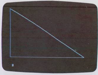
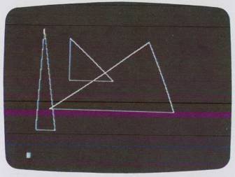
Example 9:

Draw a simple right triangle using three separate HPLOT statements on the Apple in high resolution.

Solution:

10 HGR : HCOLOR = 3
20 HPLOT 0, 0
30 HPLOT TO 0, 159
40 HPLOT TO 279, 159
50 HPLOT TO 0, 0
60 END

See Fig. 3-9.

Fig. 3-9. Plot of right triangle.

Boxes and Rectangles

Drawing rectangles requires that we pick the four corners and place them in an HPLOT TO statement. There are some surprises, however. See Example 10, p. 116.

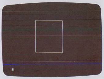
The first thing we notice is that this isn't a true square, that is, the sides don't look equal on the screen even though we know they are! The obvious reason is that an increment on the X axis is not the same as an increment on the Y axis. Here is how to fix this so your shapes are perfect. Take out a ruler and measure the sides of the square. This will vary with your particular television set. On one set this was Y = 2.5 inches (6.35 cm) and X = 2.0625 inches (5.23 cm). Now divide Y by X to get the ratio, here 2.5 / 2.0625 = 1.212. This ratio says that one step in Y gives about 1.212 times the same step in the X. Or the Y spacing is about 21 percent longer than the X spacing. The trick now is to adjust our programs by multiplying X by 1.212, or dividing Y by 1.212 just before we do the actual plotting (of course using your own constant ratio).

Example 10:

Draw a square 100 × 100 units on the Apple II in high resolution. Center the square.

Solution:

Since we know the screen is 279 by 159 we assume that the center of the screen is 140, 80 and thus make the upper left starting corner of the box 140 - (100 / 2) = 90 and 80 - (100 / 2) = 30.

10 HGR : HCOLOR = 3
20 HPLOT 90, 30 TO 190, 30 TO 190, 130 TO 90, 130 TO 90, 30
30 END

See Fig. 3-10.

Fig. 3-10. Computer plot of square.

This is all very nice, but how do we implement the ratio correcting idea into our programs? The way to do this is to make the shape size dependent on a pair of variables. At the same time make the shape's starting location on the screen a variable also. See Example 11.

Example 11:

Draw a square 100 × 100 units on the Apple II using a correction factor of 1.212 (or whatever your screen is) to remove distortion and make the shape size and the start corner variable.

Solution:

10 HGR : HCOLOR = 3 : F = 1.212	←Correction “factor” for your tv
20 XS = 100 * F
30 YS = 100
40 X = XS / 2 : Y = YS / 2
50 I = 140 : J = 80	←Screen center
60 HPLOT I - X, J - Y TO I + X, J - Y TO I + X, J + Y TO I - X, J + Y TO I - X, J - Y	←Variable-size box
70 END

See Fig. 3-11.

Fig. 3-11. Plot of square with correction factor included.

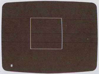
Although this program is more complicated than the one before it, notice how easy it is to move the square around or change its size. The x side is called XS and the y side is called YS. Statement 20 multiplies XS by F, our correction factor. Statement 40 makes X and Y equal to one-half the size of the x and y sides. The variables I and J are used to select where on the screen to draw the square. In this program we made I and J the center of the screen. Finally the HPLOT statement in line 60 draws the actual square, using I and J as the “reference” points, and X and Y as the sides of the square.

Example 12:

Write a program to draw four boxes of various sizes on the Apple II in high-resolution color. Use DATA statements to hold the corner coordinates of the boxes and let N equal the number of boxes.

Solution:

10 HGR : HCOLOR = 3 : F = 1.212
15 N = 4	←Number of boxes
20 FOR L = 1 TO N
25 READ I, J, XS, YS	←Location of box and its dimensions
30 X = XS * F / 2 : Y = YS / 2
35 HPLOT I - X, J - Y TO I + X, J - Y TO I + X, J + Y TO I - X, J + Y TO I - X, J - Y
40 NEXT L
45 END
100 DATA 140, 80, 100, 100	←Each data/statement holds I, J, XS, and YS
105 DATA 140, 80, 200, 15
110 DATA 50, 40, 20, 20
115 DATA 230, 60, 5, 100

See Fig. 3-12.

Fig. 3-12. Plot of four boxes.

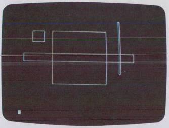
To make things even more flexible we can use the DATA statement to store the coordinates of the corners of the box. Then we can structure our program so it can display several boxes with each box described by its own DATA statement (we will extend this idea often in the text). See Example 12.

Example 13:

Write a program to draw three right triangles with angles of 30°, 45°, and 80° on the Apple II in hires.

Solution:

10 HGR : HCOLOR = 3 : F = 1.212
15 PI = 3.14159
20 N = 3	←Number of triangles
25 FOR K = 1 TO N
30 READ I, J, O, T	←Location of 90° corner, length of opposite side, angle T
35 T = 90 - T : T = T / 180 * PI
40 A = 0 / TAN (T) / F	←Finds length of adjacent side Plots a triangle
45 HPLOT I, J TO I-O, J TO O, J-A TO I, J
50 NEXT K
55 END
100 DATA 140, 80, 70, 45
105 DATA 240, 120, 200, 30
110 DATA 50, 150, 30, 80

See Fig. 3-13.

Fig. 3-13. Plot of three right triangles.

The FOR…NEXT loop in statement 20 causes the program to read a DATA statement and assign the values in it to the variables I and J (the location of the box center) and then XS and YS (the length of the sides of the box). Next, in statement 30 we multiply XS by the correction factor F and divide XS and YS by 2 to get the half-side length. Finally, statement 35 is like the previous program statement 60; it plots the box shape according to the variables I, J, X, and Y. The loop then repeats for the next N — 1 boxes.

Triangles

Triangles (of the right-angle type) may be generated by specifying a corner location (I, J) for positioning the triangle, an opposite side (O), and an angle (call it T) in the range of 0° to 90°. We can then use the formula

A = 0/tan T

to find the length of the adjacent side (A) and then divide by F to correct for screen distortion. Since T is specified in degrees we can convert to radians with the formula:

T_r = T_d/180/π

where π = 3.14159. See Example 13, p. 119.

The first two values in the DATA statements are the location of the right-angle (90°) corner, the third value is the length of the opposite side, and the last value is the angle in degrees. Other than that the program is just like the previous one. You can add more triangles by adding more DATA statements and adjusting N.

Regular Polygons

Polygons are those closed figures having three or more sides and each side may be any length. The polygons we are most familiar with are the “regular” polygons, i.e. those with equal-length sides, such as the pentagon, hexagon, and so on.

To draw polygons on a computer with vector graphics is similar to the way we plot circles, except instead of plotting points we draw lines. See Example 14, p. 121.

Some oddities worth mentioning in the program—the FOR …NEXT loop which generates the angles T is:

FOR T = A1 TO A2+.01 STEP INC

The + .01 is an increment that must be added to A2 to ensure that the loop doesn't skip the last value of T (6.28313), which can happen due to rounding errors.

Example 14:

Write a program to draw a pentagon (five sides), hexagon (six sides), and an octagon (eight sides) on the Apple II in hires. Use the circle generation approach and make the polygons concentric (all have the same center). Let N = number of sides, L = number of polygons, and R = radius of polygon.

Solution:

10 HGR : HCOLOR = 3 : PI = 3.14159
15 F = 1.212 : A1 = 0 : A2 = 2 * PI
20 L = 3
25 FOR S = 1 TO L
30 READ I, J, R, N
35 INC = (A2 - A1) / N
40 FOR T = A1 TO A2 + .01 STEP INC
45 X = R * SIN(T)
50 Y = R * COS(T) / F
55 IF T = A1 THEN HPLOT I + X, J + Y
60 HPLOT TO I + X, J + Y
65 NEXT T : NEXT S
70 END
100 DATA 140, 80, 50, 5
105 DATA 140, 80, 60, 6
110 DATA 140, 80, 70, 8

See Fig. 3–14.

Fig. 3-14. Plot of three concentric polygons.

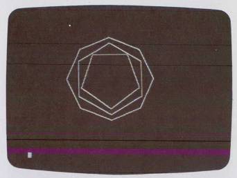
The variable F adjusts the polygons for screen distortion. The IF…THEN statement at line 55 is needed because of the nature of the HPLOT TO statement, and it locates the first dot location for the later line vectors.

Circles

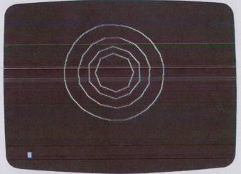
We can produce a convincing display of the beauties of math by noting that as the number of sides in the polygon increases, the more the polygon resembles a circle (Example 15).

Example 15:

Draw four concentric circles, using the “polygon” approach, starting with 8 sides, then increasing to 10, 15, and finally 45 sides. Have the radius of each circle increase as the number of sides increases so we can see the differences.

Solution:

10 HGR: HCOLOR = 3: PI = 3.14159
15 F = 1.212: A1 = 0: A2 = 2*PI
20 L = 4
...
{as in previous program}
...
...
100 DATA 140,80,30,8
105 DATA 140,80,40,10
110 DATA 140,80,55,15
115 DATA 140,80,75,45

See Fig. 3-15.

Fig. 3-15. Polygon approach to plotting circles.

Now let's review what we have covered in this section. The concepts for drawing simple geometric shapes have been shown. We have also seen the techniques for making our shapes “relocatable” and for making them change size easily.

In the next section we shall explore concepts for making figures for game programs—figures that can be moved, bounced, or shot across the screen.

---

Return to Table of Contents | Previous Section | Next Section