PLOTTING
To plot on a graphics computer is to place a dot or square somewhere on the screen of the computer. The size of the dot, whether it is colored or just black and white, and so on, depend on the type of computer you are using. How you get the dot plotted on the screen also depends on the type of computer. In general, home computers use special graphics instructions to get the dot plotted on the screen. These instructions are called graphics statements. Usually they are part of the BASIC programming language of the machine, but in some cases (RCA VIP) they may be assembly language instructions.
As an example, to plot in the TRS-80 we use the statement SET X, Y (where X and Y specify the horizontal and vertical location for the dot on the screen matrix). To remove the dot the statement RESET X, Y is used.
On the Apple II in the high-resolution mode we use the statement HPLOT X, Y to plot a dot. The color of the dot must first be set with the HCOLOR = statement. In the low-resolution mode on the Apple II we use the statement PLOT X, Y to plot a color square on the screen. The color of the square is set previously with the COLOR = statement.
There are several uses for the plot instruction, including the plotting of equations, the drawing of pictures, and so on. Here we will explore the plotting of equations on the Apple in the high-resolution mode.
Plotting Equations
One of the most useful applications of the graphics computer is its ability to plot the graph of a complex equation. Besides removing the drudgery of plotting equations by hand, using the graphics computer to automatically plot allows the viewer to “see” the insides of an equation as it is drawn out onto the screen. For example, imagine plotting the path of a swinging pendulum on the screen, the trajectory of a model rocket, the three waveforms of a biorhythm chart, the delay of a pulse, and so on.
The generation of the graph of an equation is accomplished by simply placing the equation itself inside some kind of a programmed loop, such as a FOR…NEXT loop in BASIC. The purpose of the loop is to generate values for the horizontal axis (X) and feed them to the equation. The equation then takes these values and produces the corresponding value for the vertical axis (Y). The X and Y pair is then used inside a PLOT statement (or HPLOT or whatever) to make one point of the graph appear on the screen.
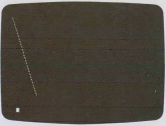
A good place to begin for an equation plotting program is with a simple equation for a straight line (see Example 1, p. 105). Recall that the equation for a straight line is Y = mX + b.
As you can see the graph of the equation is upside down. This is because on the Apple in high-resolution 0, 0 is the upper left corner of the screen and the Y axis extends down the screen to 159.* The X axis extends from zero on the left to 279 on the right.
The graph of the equation can be “flipped” over by simply changing the equation to Y = 159 - (3*X + 10). Since Y must not exceed 159 or be less than 0 we must restrict the range of X (-3 < X < 50).
Example 1:
Generate the graph of the straight-line equation
y = 3x + 10 (x = 0 to 50)
on the Apple II in the high-resolution mode.
Solution:| ←Switches Apple into high-resolution graphics mode | |
10 HGR: HCOLOR = 3 |
←Sets color to white |
20 FOR X = 0 TO 50 |
←start the loop |
30 Y = 3*X + 10 |
←Our equation |
40 HPLOT X, Y |
←Plot it |
50 NEXT X |
|
END |
See Fig. 3–1.
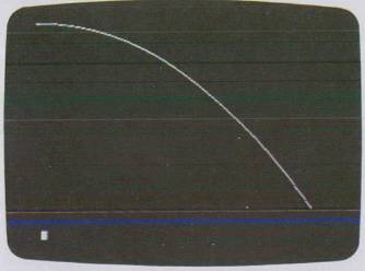
Nonlinear equations that form interesting curves are the next logical type of equation to try graphing with a plotting program. See Example 2, p. 106.
Here the magic term X^2 makes the Y values grow faster than the X values and hence a curve is formed. The trick to getting this to work on the computer is to divide the equation by 490 in order to keep Y from growing beyond 159. We can flip the graph over with 30 Y = 159 - (X^2/490).
Example 2:
y = x2 (x = 1 to 279)
on the Apple II in hires (high resolution).
Solution:
10 HGR: HCOLOR = 3

20 FOR X = 1 TO 279

30 Y = (X^2)/490

40 HPLOT X, Y

50 NEXT X

60 END
See Fig. 3-2
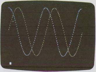
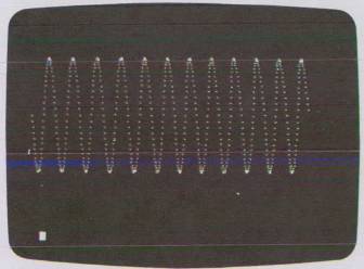
Harmonic motion, interference, sinusoidal oscillation, and other wavelike phenomena can easily be displayed on the screen of the computer. See Example 3, p. 107.
Here is how the program works. Statement 10 puts us in the high-resolution mode, sets the radius R to 79, and sets the constant two-pi (TPI) to 6.28318. Next we enter a FOR…NEXT loop which produces values of I degrees from 0 to 720. Next in statement 30 we divide I by 2.58 so that X varies from 0 to 279 for the HPLOT statement (remember the rules).
The expression (I/360*TPI) in statement 40 is the formula for converting degrees (I) to radians. The formula is inside the SIN function, so we get Y1 to equal to the sine of I degrees, which varies from -1 to + 1. Multiplying by 79 sets the maximum and minimum peaks for the sine plot of Y1 and Y2. Next we set the HCOLOR to green with HCOLOR = 1 and finally the great HPLOT statement : HPLOT X, 80 - Y1 actually plots the equation Y1 on the screen (naturally turning Y1 upside down with 80 - Y1.
Example 3:
Plot two cycles (x = 0° to 720°) of the equations:
y1 = sin x
y2 = cos x
on the Apple computer in high-resolution color. Make the curve out of dots and make equation y1 plot in green and y2 in violet. Use the slow but simple and effective “brute-force” approach where the limits of the FOR…NEXT loop are in degrees.
Solution:
| ←Radius | |
10 HGR : R = 79: TPI = 6.28318 |
←Two pi |
20 FOR I = 0 to 720 |
←Loop makes 1 = 0 to 720 |
30 X = 1/2.58 |
|
40 Y1 = R*S IN(1/360*TPI) |
|
50 HCOLOR = 1: REM GREEN DOTS |
|
60 HPLOT X, 80–Y1 |
|
70 Y2 = R*COS(I/360*TPI) |
|
80 HCOLOR = 2: REM VIOLET DOTS |
|
90 HPLOT X, 80–Y2 |
|
100 NEXT I |
See Fig. 3-3.
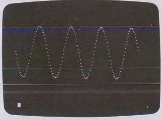
Example 4:
Plot four cycles of the equation:
y = sin t (t = -4π to + 4π)
on the Apple computer in high-resolution color graphics using the “N = number of points” plotting method. Use 180 points for N, and use radians instead of degrees.
Solution:
10 HGR: HCOLOR = 3: PI = 3.14159 |
|
15 A1 = -4*PI |
←Lower limit in radians |
20 A2 = 4*PI |
←Upper limit in radians |
25 N = 180 |
←Number of points |
30 R = 50 |
←Radius |
35 INC = (A2 - A1)/N |
←Increment |
40 F = 279/(A2 - A1) |
←Factor (multiplier) to get X |
45 FOR I = A1 TO A2 STEP INC |
|
50 X = I * F |
|
55 Y = R * SIN(I) |
|
60 HPLOT 140 + X, 80 + Y |
|
65 NEXT I |
|
70 END |
See Fig. 3-4.
Statement 70 generates the cosine of I (which, as electronics buffs know, leads the sine by 90°). Last, the equation of Y2 is plotted by statement 90 and we loop to the next value for I degrees.
Note that the plot in Fig. 3-3 is not smooth. Further, from a time standpoint the program took over 30 seconds to draw out on the screen. This is due to the fact that we are attempting to plot so many points (1440 here).
A much better way to plot a trigonometric function involves specifying the number of points to plot. See Example 4, p. 108.
Here is how this program works and why it is better than the previous brute force program. Statement 10 switches us into graphics, sets the color to white, and sets the variable P1 to 3.14159. Statements 15 and 20 set A1 and A2 to equal the limits of the sine wave in radians (multiples of π). Statement 25 sets N to 180, and statement 30 sets the radius R to 50. Statement 35 then takes these limits and produces the variable INC, which will be used as the step size for the upcomin FOR…NEXT loop! Statement 40 produces the multiplier F that will be used later to generate values of X for the screen from values of I.
In statement 45 we begin the main FOR…NEXT loop that plots out our sine wave. Note the loop limits are A1 to A2 so we can easily put other functions inside the loop and the loop increment is INC. In statement 50 we first produce our value of X for the screen from the loop index I (remember I is in radians and the screen is not). Then in statement 55 we generate our corresponding Y value using the trigonometric SIN function. The variable R multiplies Y to set the “peak-to-peak” size of the function.
Statement 60 is different from previous HPLOTs in that we define the center of the screen to be 140, 80 and add the values of X and Y to these constants to get the actual plot point. We can do this because the loop index is in radians and negative values of X and Y are produced from the SIN function.
This program is extremely flexible because we can change so many things so quickly. For example, to add more plotting points simply make N larger in statement 25; or to increase frequency (i.e. add more values on the screen) simply make A1 and A2 larger. See Example 5, p. 110.
Polar Plotting
Plotting equations in “polar” form makes it very easy to plot circles and ellipses on the computer. In fact very beautiful patterns can be generated from polar equations by repeated plotting of the same equation with a slight shift occurring in one parameter. In a polar equation we generate values for an angle in radians (preferably 0 to 2π or 0° to 360°). Then we use the values for the angles inside the function that we wish to plot. Finally, we use a transformation formula to get the proper X, Y values for a Cartesian coordinate system as on the computer screen. The previous sine wave program was close to a polar plot. The next program shows how to form a circle, by a polar equation. See Example 6.
Example 5:
Increase the frequency (number of crests on the screen) to 12 and increase the number of points N to 720. See how much longer the plot takes.
Solution:
10 HGR: HCOLOR = 3: PI = 3.14159 |
|
15 A1 = -12 * PI |
←New lower limit |
20 A2 = 12 * PI |
←New upper limit |
25 N = 720 |
←New number of points |
ċ |
|
... |
|
... |
|
{as in previous program} |
|
... |
|
... |
|
70 END |
See Fig. 3-5.
Example 6:
Graph the polar equation for a circle of radius
r = 50 (0 to 2π radians)
on the Apple in high-resolution color. Use N to specify the number of points as 32.
Solution:
10 HGR : HCOLOR = 3 : PI = 3.14159

15 A1 = 0

20 A2 = 2 * PI

25 N = 32

30 R = 50

35 INC = (A2 - A1) / N

40 FOR I = A1 TO A2 STEP INC

45 X = R * SIN(I)

50 Y = R * COS(I)

55 HPLOT 140 + X, 80 + Y

60 NEXT I

65 END
See Fig. 3-6.
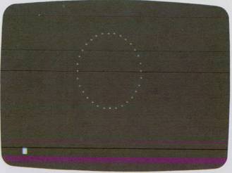
As you can see we almost get a perfect circle. Try the above program a second time, only increasing the number of points to 64, and notice that the dots tend to disappear.
Now, in case you didn't know it, the actual function we plotted in our previous program was the equation r = 50. What if we change the equation so r is no longer a constant? For example, we could have r = cos t. What kind of plot do you think will occur? See Example 7, p. 112.
Example 7:
Plot the graph of the four-leaf “rose curve” polar equation
r = a cos 2t (t = 0 to 2π, a = 50)
using the relations
x = r sin t y = r cos t
on the Apple II in high-resolution color.
Solution:
10 HGR : HCOLOR = 3 : PI = 3.14159 |
|
15 A1 = 0 : A2 = 2 * PI |
|
20 N = 90 : A = 50 |
|
25 INC = (A2 - A1) / N |
|
30 FOR I = A1 TO A2 STEP INC |
|
35 R = A * COS(2 * 1) |
|
40 X = R * SIN(I) |
←Conversion from polar to Cartesian coordinates |
45 Y = R * COS(I) |
|
50 HPLOT 140 + X, 80 + Y |
|
55 NEXT I |
|
60 END |
See Fig. 3-7.
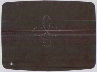
This program is similar to the previous one except we use the cosine function (COS) to generate the value of R. As you can see in Fig. 3-7 the rose curve has four “petals” to it. There are actually whole families of rose curves that can be plotted on the computer. The equations for these can be found in any standard math reference book.
To add more points to the rose curve simply make N in statement 20 larger; to increase the diameter of the curve make A in statement 20 larger. Be careful because the program doesn't check the values of X and Y before they are plotted by statement 50, and if they are too large or too small, an error message will occur.
Return to Table of Contents | Previous Section | Next Section